Martin Yeo

Excel: Advanced Scoring

Run numbers through a complex grading system without resorting to enormous nested IF() statements…

---

Simple IF() statements can be used to assign a grade based on a value, for example:

=IF(A1<50,”Bad”,”Good”)

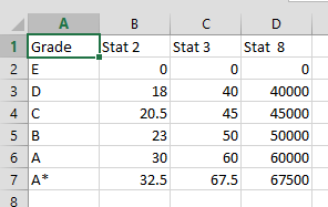
However, as one adds more grading bands and possibly more than variable to assess, these statements will become much larger and more difficult to maintain. It is much better to make use of a table against which grades can be looked up. Here is an example:

This table has 6 grades - E to A* - and thresholds for 3 stats that must all be reached before the relevant grade is achieved. We now need a formula that will be able to identify the highest row number where all 3 threshold have been met, and return the appropriate grade from this row number. INDEX() can easily perform the second part of that sentence:

=INDEX($A$2:$A$7,???)

So how do we return the correct row number? As is often the case when using Excel to find a row using a number of criteria, SUMPRODUCT(MAX()) is the answer. Within the MAX() statement we place a number of boolean statements. SUMPRODUCT() allows us to assess whole arrays in each of these booleans, so we use them to test a number against a whole column of the grading table:

--(53800>=$D2:$D7) returns {1,1,1,1,0,0}

When we multiply several booleans together, each checking an array of the same rows but a different column, we end up with a single array of TRUE’s and FALSE’s (represented as 1 or 0), e.g. {1,1,0,0,0,0}. Multiply this array together with the actual row numbers to get an array of row numbers where all thresholds have been met:

{1,1,0,0,0,0}*ROW($A$2:$A$7) returns {2,3,0,0,0,0}

Because we have placed this within a MAX() statement, the highest row number is returned and passed into the INDEX() statement. When using this method, the grades must be sorted ascending in their table - attempting the reverse using a MIN() statement will only work when the best grade has been achieved ( otherwise MIN() will return a 0). Here is an example of the full formula:

=INDEX('Scoring Table'!$A$2:$A$7,SUMPRODUCT(MAX(--($D$7>;='Scoring Table'!$B$2:$B$7)*--($D$8>;='Scoring Table'!$C$2:$C$7)*--($D$9>;='Scoring Table'!$D$2:$D$7)*ROW('Scoring Table'!$A$2:$A$7))))

Click here to see this method in action.